Plotting one continuous fields with shading and another discrete one with points
draw_2D_shad_contdisc(ncfiles, values)
ncfiles= [contfilen];[contvarn];[dimxvarn];[dimvvarn];[dimvals]@[discfilen];
[discvarn];[dimxvarn];[dimyvarn];[dimvals] files and variables to use
[contfilen]: name of the file with the continuous varible
[contvarn]: name of the continuos variable
[dimxvarn]: name of the variable with values for the x-dimension
[dimvvarn]: name of the variable with values for the y-dimension
[dimvals]: ',' list of [dimname]|[value] values to slice the variable:
* [integer]: which value of the dimension
* -1: all along the dimension
* -9: last value of the dimension
* [beg]@[end]@[inc] slice from [beg] to [end] every [inc]
* NOTE, no dim name all the dimension size
[discfilen]: name of the file with the discrete varible
[discvarn]: name of the discrete variable
* NOTE: limits of the graph will be computed from the continuous variable
values=[vnamefs]:[dvarxn],[dvaryn]:[dimxyfmt]:[colorbarvals]:[sminv],[smaxv]:
[discvals]:[figt]:[kindfig]:[reverse]:[mapv]:[plotrange]:[close]
[vnamefs]: Name in the figure of the variable to be shaded
[dvarxn],[dvaryn]: name of the dimensions for the final x-axis and y-axis at
the figure (from contfilen)
[dimxyfmt]=[dxs],[dxf],[Ndx],[ordx],[dys],[dyf],[Ndy],[ordx]: format of the
values at each axis (or 'auto')
[dxs]: style of x-axis ('auto' for 'pretty')
'Nfix', values computed at even 'Ndx'
'Vfix', values computed at even 'Ndx' increments
'pretty', values computed following aprox. 'Ndx' at 'pretty' intervals (2.,2.5,4,5,10)
[dxf]: format of the labels at the x-axis ('auto' for '%5g')
[Ndx]: Number of ticks at the x-axis ('auto' for 5)
[ordx]: angle of orientation of ticks at the x-axis ('auto' for horizontal)
[dys]: style of y-axis ('auto' for 'pretty')
[dyf]: format of the labels at the y-axis ('auto' for '%5g')
[Ndy]: Number of ticks at the y-axis ('auto' for 5)
[ordy]: angle of orientation of ticks at the y-axis ('auto' for horizontal)
[colorbarvals]=[colbarn],[fmtcolorbar],[orientation]
[colorbarn]: name of the color bar
[fmtcolorbar]: format of the numbers in the color bar 'C'-like ('auto' for %6g)
[orientation]: orientation of the colorbar ('vertical' ['auto'], 'horizontal')
* NOTE: single 'auto' for 'rainbow,%6g,vertical'
[smin/axv]: minimum and maximum values for the shading or string for each for:
'Srange': for full range
'Saroundmean@val': for mean-xtrm,mean+xtrm where
xtrm = np.min(mean-min@val,max@val-mean)
'Saroundminmax@val': for min*val,max*val
'Saroundpercentile@val': for median-xtrm,median+xtrm where
xtrm = np.min(median-percentile_(val),percentile_(100-val)-median)
'Smean@val': for -xtrm,xtrm where xtrm = np.min(mean-min*@val,max*@val-mean)
'Smedian@val': for -xtrm,xtrm where
xtrm = np.min(median-min@val,max@val-median)
'Spercentile@val': for -xtrm,xtrm where
xtrm = np.min(median-percentile_(val),percentile_(100-val)-median)
[discvals]= [type],[size],[lwidth],[lcol] characteristics of the points for the discrete field
[type]: type of point. Any marker from matoplib must be filled !
[size]: size of point
[lwidth]: width of the line around the point
[lcol]: color of the line around the point
* 'auto': for [type]='o', [size]=5, [lwdith]=0.25, [lcol]='#000000'
[figt]: title of the figure ('!' for spaces)
[kindfig]: kind of figure output (ps, png, pdf)
[reverse]: Transformation of the values to plot
* 'transpose': reverse the axes (x-->y, y-->x)
* 'flip'@[x/y]: flip the axis x or y
[mapv]: map characteristics: [proj],[res]
see full documentation: http://matplotlib.org/basemap/
[proj]: projection
* 'cyl', cilindric
* 'lcc', lambert conformal
[res]: resolution of the coastaline data:
* 'c', crude
* 'l', low
* 'i', intermediate
* 'h', high
* 'f', full
[plotrange]: range of the plot
'strict': map covers only the minimum and maximum lon,lats from the
locations of the discrtete points
'sponge,'[dlon],[dlat]: map covers an extended [dlon],[dlat] from the
minimum and maximum lon,lats from the locations of the discrtete points
'fullcontinuous': map covers all the shadding area
'lonlatbox,[lonSW],[latSW],[lonNE],[latNE]': plotted map only covers a lon,lat box
[close]: Whether figure should be finished or not
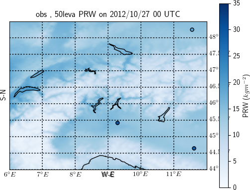
$ python ${pyHOME}/drawing.py -o draw_2D_shad_contdisc -f 'simcdx_vars_cape_50lev_assigned.nc;PRW;LON;LAT;
Time|23,time|23,west_east|-1,south_north|-1@all_sounding_1D.nc;prw;stslon;stslat;time|14,lon|-1,lat|-1'
-S 'PRW:west_east,south_north:auto:Blues,auto,auto:0.,35.:auto:obs!,!50leva!PRW!on!2012/10/27!00!UTC:png:
None:cyl,i:lonlatbox,6.,44.,12.,48.5:yes'